lidar-technology

OK Osaki Tsuji Boehm, Liesenberg- Appraisal of LIDAR measurements for monitoring tropical peatlands - 14112022 - updated_14.07.2023

[A1] [VL2] [A3] [VL4] Chapter 11  Appraisal of LiDAR measurements for monitoring tropical peatlands

Hans-Dieter Viktor Boehm^1* Veraldo Liesenberg²

1. Kalteng Consultants, Kirchstockacher Weg 2, 85635 Hoehenkirchen near München, Germany
2. Santa Catarina State University, Av. Luiz de Camoes, 2090, 88520-000 Lages, Brazil

*Corresponding Author: viktorboehm@t-online.de

Key words:

Biomass, Digital surface model (DSM), Digital terrain model (DTM), Environmental verification, Geographic information system (GIS), LiDAR, Peat-Dome, Surface and terrain model, Topography

Abstract

Tropical peat swamp forests are important for their rich biodiversity and serve as a huge carbon pool. However, these endangered environments are decreasing due to deforestation, conversion into farmland, excessive draining, the use of shifting cultivation on a large scale, illegal logging, forest degradation and palm oil plantations. Airborne laser scanning (ALS), also termed airborne light detection and ranging (LiDAR), is currently a good single sensor to investigate geophysical parameters in remote tropical rainforest areas (e.g., tree canopy height, which is strongly correlated with aboveground biomass).

This chapter aims to describe the LiDAR system and to present the applicability of LiDAR data to environmental work in tropical peatlands of Central Kalimantan, Indonesia. Several channels of the EX-Mega Rice Project (EMEP) and Sebangau National Park with peat swamp forest (PSF) will be presented. LiDAR surveys were performed by helicopter surveys in 2007 and 2011, allowing us to perform change detection that highlighted vegetation dynamics and subsidence of peatlands. LiDAR shows promising opportunities for reducing emissions from deforestation and forest degradation (REDD) and environmental assessments.

11.1 Introduction

A LiDAR system can rapidly transmit laser pulses at both daytime and nighttime. The pulse is, therefore, a reflection of both landscape and man-made features. The known speed of light and the measured time interval of the laser pulses from transmission to return allow the determination of distances (Asner et al., 2012, Liesenberg et al., 2013). An aerial survey can be performed either by a fixed-wing airplane, helicopter, or drone with LiDAR equipment installed, which includes an inertial navigation system (INS) with gyros for measuring the platform vibrations and a GPS[A5] [VL6] [VL7] . The result is an innovative tool for studying the ground surface and all objects on it. Possible applications include hydrology, topography, archelogy, measurements of peat dome, extraction of tree height, estimation of Above-Ground Biomass (AGB), etc. (Takahashi and Yonetani, 1997, Liesenberg et al., 2013, Engelhart et al., 2012, Hajnsek et al., 2009, Kronseder et al., 2012, Schlund et al., 2016, 2021, Osaki and Tsuji, 2016). A LiDAR survey provides data beyond that of a conventional survey with traditional cameras and even field measurements (which are time-demanding and costly).

In summary, digital elevation models can be derived from LiDAR point clouds and used for a wide variety of tasks. Another derived product is named the canopy height model (CHM) and can be used to extract objects such as buildings and even individual trees. This product also allows us to derive vertical height metrics that may serve as input data in mathematical models to retrieve volume. On the other hand, the digital terrain model (DTM), which is one of the main products derived from LiDAR, includes the design of infrastructure such as roads and water canals (Boehm et al., 2010).

The accuracy of the surface generated depends on several factors defined during LiDAR data acquisition, such as frequency and point density (i.e., 1-10 m²). Generally, it lies between 15 cm in elevation (z), which seems to be optimal for agricultural planning, peatland research, firer analysis (Boehm et al., 2011a), river catchment surveys, flood mapping and mining surveys (Boehm et al., 2011, 2012, Sweda et al., 2012, Osaki and Tsuji, 2016). Interestingly, eroded areas can be accurately surveyed, even through a thick, dense grass layer.

The motivation of the abovementioned research involving LiDAR surveys was to obtain a better understanding of the tropical peatlands in Central Kalimantan to analyze the topography, tree heights, biomass, different peat dome profiles, carbon budget and subsidence of peatlands (Silvius, 1989, Jaenicke et al., 2008, Boehm et al., 2012, Hooijer et al., 2012, Sweda et al., 2012, Liesenberg et al., 2013) with this technology. A review of some applications of the helicopter surveys made with LiDAR over three tropical peatland areas during two helicopter flight campaigns in 2007 and 2011. First, the concept of generating DEMs is provided. Second, the LiDAR system is integrated into a helicopter. Then, LiDAR acquisition and preprocessing steps, including the results of the surveys, are presented. Finally, further perspectives and open research questions are presented as final remarks.

11.2 Generation of digital elevation models

The eye-safe laser in the system has a very narrow beam called small-footprint LiDAR, which means that it can penetrate gaps in vegetation to reach the ground surface through tree gaps or other openings that are typically not visible from traditional stereo imagery. This penetration allows for an accurate determination of ground levels in vegetated areas. The laser also reflects above-ground objects, giving positions and heights of power lines and power poles, high and low vegetation, buildings, bridges, and fences, among others, building up a three-dimensional (3D) picture of the survey area. In addition, multiwave technology can also provide differentiated information about single trees or a forest canopy. We used the first and last laser pulses for tree analysis, but the multiwave information was stored (Boehm et al. 2011).

Due to the instrumentation in the LiDAR system that provides accurate position and attitude information for the laser points and an installed camera, very few ground control points are needed, which means that accurate surveys are possible in inaccessible areas. These include quarries, wetlands, floodplain measurements, etc. (Liesenberg et al. 2013). The LiDAR data can be processed and then made available with a geo-referenced position for visualization in a geographical information system (GIS). The LiDAR data overcome the common digital elevation model (DEM) by refining it into a digital surface model (DSM) with buildings and trees and a DTM with the topography of the landscape. The canopy height, also known as the normalized DSM (CHM or nDSM), can be obtained as follows: CHM = DSM – DTM.

11.3 LiDAR-System integrated on helicopters

Using airborne LiDAR, the topography of Central Kalimantan peatlands was measured to obtain both the DSM and DTM (Figs. 11.1 to 4). The flight was approximately 500 m above ground, and the footprint was 500 m.

With this information, hydrology models of peatland and the retrieval of biomass of Peat Swamp Forest (PSF) can be analyzed (Liesenberg et al., 2013). The data resolution depends on the type of LiDAR scanner and the flight height of the aircraft (helicopter, fixed-wing airplane or drone)[A8] [VL9] .

Sometimes such a LiDAR-sensor system can also be combined with a high-resolution ortho-photo RGB camera and a hyperspectral scanner. For example, we used a high-resolution Hasselblad camera with a Riegl Laser-Scanner (RIEGL Laser Measurement Systems GmbH, Horn, Austria).[A10] [VL11] 

[A12] [VL13] 

Fig. 11.1. Principle of a Laser Scanner – LiDAR System.

Fig. 11.1 shows the principle of a laser scanner to archive good information from peatlands. The processing with filtering of the achieved data is very important to obtain a correct high-resolution 3D-peatland-GIS. Currently, many companies offer laser scanner acquisition services under variable prices according to survey characteristics. The results described here were possible using a helicopter and adapting the LiDAR system using an attached platform in the landing skids (Fig. 11.2) or using the platform on the back side of the engine (Fig. 11.3).

Fig. 11.2. A LiDAR system integrated under the bottom of a Bell helicopter, 2007

Fig. 11.3. A LiDAR system integrated in the back on a stabilized plate of a BK117 helicopter, 2011

Additionally, an internal navigation and flight management system are necessary for a LiDAR scanner system. A LiDAR scanner system [A14] [VL15] can be combined with a GPS antenna L1/L2 band, a DGPS ground station, and several recorders to obtain high-resolution accurate time and location information.

11.4 LiDAR acquisition and preprocessing

The LiDAR transects in Kalimantan (Indonesia) were surveyed twice by Kalteng Consultants and Milan Geoservice GmbH (Fig. 11.4) from August 5 to 7, 2007, and August 4 to 5, 2011, using a Riegl LMS-Q560 Laser Scanner System. It was attached to a Bell 206 helicopter for the first flight trial and a BK117 helicopter for the second flight trial[A16] [VL17] . The nominal height was on average 530 m for both surveys. A differential global positioning system (DGPS) reference station was mounted at the airport of Palangkaraya City, considering an elevation of 25.0 m or 82 feet. The position and orientation of the LiDAR system on the helicopter were measured by an inertial navigation system (INS) and a differential GPS located on the tail boom, respectively, on the cockpit roof at 256 Hz. A complete description of the LiDAR survey can be found in (Boehm et al., 2010, and 2011). The technical details of the LiDAR systems are further detailed in Table 11.1.

Table 11.1. Specifications of the airborne LMS-Q560 LiDAR (Riegl) system and its data products

Note: for the flight measurements taken in *2007 and **2011.

Ground backscattering passing through dense PSF amounted from 1% to 3% of the total laser beams. The processed laser beams were classified into ground surface and aboveground classes using a terrain-adaptive bare earth algorithm for both dates. The algorithm is integrated with Cloud Peak software (LASEdit) and IDL software used by Milan, provides an unsupervised classification of the cloud points, and adapts it to a hypothetical bare earth condition. First, the triangular irregular network (TIN) was constructed based on a Delaunay triangulation. Then, a square grid of pixels was extracted for each TIN using linear interpolation for both ground and aboveground layers on both acquisition dates. Next, the classified laser representing the ground surface was converted into the DTM and DSM, both with a spatial resolution of 1 m. The difference between the DSM and DTM provided us with the CHM.

11.5 LiDAR surveys in Central Kalimantan

The three selected test sites on Sebangau National Park and in the Mawas area are relatively flat. According to Shepherd et al. (1997) and Page et al. (1999), the peat thickness of the Sebangau test site varies from 0 to 12 m. Estimates conducted by Jaenicke et al. (2008) using GIS techniques showed that the peat thickness varies from 0 to 18 m at Mawas sites. The climate of the entire study area, following the Köppen climate nomenclature, is humid tropical rainforest (Af).

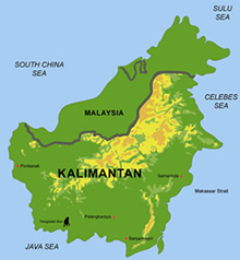
Fig. 11.4. Location of the study area in Central Kalimantan, Indonesia (top) and location of the three selected test sites (below). The yellow rectangle shows the location of Palangkaraya City. The solid yellow lines indicate the LiDAR transects (A). The lower part of the image indicates the following: Mawas km228 south of the equator (a), Mawas km238 (b) and Sebangau (c). Each test site is shown in more detail in the Landsat-7/ETM+ images acquired on August 5, 2007 (3R4G5B).

Fig. 11.5 shows the LiDAR transect in more detail with the raw count lines at meter intervals showing the typical flat characteristics of the PSF landscape. The resulting height profiles are shown in Fig. 11.6.

Fig. 11.5. LiDAR-DTM of Sebangau Nat. Laboratory transect with 1 m contour lines; transect begins at the river with 15 m altitude, and at the end, it is at a 25 m altitude superimposed on a Landsat image. The LiDAR transect width is 500 m. On the left lower corner are visible burnt scars from 1997. The violet in the image is the Sebangau catchment, black is the river, and green is peat swamp forest, which contains some roads used for logging.[A20] [VL21] 

Fig. 11.6. LiDAR-DTM of Sebangau Nat. Laboratory transect with ground PSF plots of 50 m x 50 m measurements made in Aug. 2011. The image above shows the peat surface profile.

Field measurements are also performed over certain transects with special attention to forest height and diameter at breast height (DBH; Fig. 11.7) measured close to the Japanese flux tower (Fig. 11.8). Such measurements were collected from several field sample plots along the main transect shown in Fig. 11.9. The resulted measurements were useful to validate height metrics extracted from the LiDAR measurements (Fig. 11.10) and also very useful to estimate the ABG (Boehm et al., 2012) and leaf area index (LAI).

Fig. 11.7. DBH and tree height field measurements (Fig. 11.12) in the Sebangau Cimtrop peat swamp forest transect for LiDAR verification of the tree height collected in August 2011.

Fig. 11.8. Ortho-Photo of Sebangau Cimtrop peat swamp forest transect. Left: PSF with a camp; right: Japanese tower for measuring atmospheric data.

Fig. 11.9. Sebangau LiDAR-DTM Track with peat dome approx. 26 m altitude after 12 km LiDAR-DTM with 25 1-ha sample plots (100 m x 100 m) each extend 500 m to the south; Remark: along the transect, the steps are approx. 600 m long © 100 m x 100 m

Anor LiDAR application was selected from the EMRP area in the so-called Blocks A + E.

Fig. 11.10. Average and maximum tree height for the Sebangau Cimtrop transect

Average tree height without the peat surface. A strong relationship between tree height and peat slope exists. At km822.3, we have the tallest average trees at 17.1 m. Much water and good soil nutrition are available here. At km 819.4, we found the lowest average tree height value of 12.6 m. The tree heights increase as they were closer to the dome[A22] [VL23] , which may be caused by low-intensity logging. No railway transect was found in the last three LiDAR measurements. The steepest peat surface is at km 822 with 0.7 m-0.8 m for a 600 m path length, which is approx. 0.13% max. slope. The average tree height at 12 km is 14.6 m. The Avg. + Max. tree height, up to 37.3 m at the slopes of the peat dome, are at km 822[A24] [VL25] .

The ground field measurements allow us to assess the correlation of the DBH to tree height. Fig. 11.12 shows the average tree heights for trees at 20 cm and the average tree height of all measured trees, which are represented by black stars and blue diamonds, respectively. In comparison, the LiDAR average data for the 52 plots are shown as line-columns. LiDAR monitoring does not observe the smallest trees; therefore, for comparison reasons, we used this approach only with trees at 20 cm in the collected field data. The respective LiDAR-CHM data are shown in Fig. 11. 11 for the 52 plots. We analyzed the maximum, average-dominant (using a filtering method with a window of 10 x 10) and average tree heights for the 52 plots, including the burn scar from 1997 at the end of the transect.

Fig. 11.11. LiDAR measurements of PSF max, avg-dominant and avg tree height (CHM) in Sebangau transect 2007 with 52 plots up to the burnt scar, showing the tree heights in y-axis and the samples in x-axis.

There is a variation in tree heights between the different PSF types defined by (Shepherd et al., 1997): riverine forest (relatively small trees at the beginning), mixed pole forest (tall forest near the highest peat slope), low pole forest (in the middle), tall pole forest (near the end) and the burn scar from 1997 (at the end).

Fig. 11.12. Research area: Sebangau CIMTROP transect with 52 1 ha plots; field measurements and LiDAR-CHM

Fig. 11.13 shows the aboveground biomass (AGB) methodology to combine the measurements from the ground survey with those of the 2011 LiDAR survey. The CHM was calculated by subtracting the DTM from the DSM, and Gaussian filtering was applied to smooth the CHM with less noise and more realistic trees. We used a local maxima method to find the treetops (Hyyppä et al., 2001) and searched in a window of 5 by 5 or 3 by 3 pixels for the highest point and then determined the DBH. We found little information about allometric equations suitable for PSF in the literature. Chave (Chave et al., 2005) reported a correlation between AGB and DBH for humid tropical forests.

Fig. 11.13. Schematic diagram of the LiDAR data processing flow applied to this study

Fig. 11.14. DTM and CHM of a sample plot for 2007 and 2011 located at a burned scar area inside Sebangau National Park. Subsidence 2007 and 2011, left; regrowth 2007 and 2011, right.[A26] [VL27] 

Fig. 11.14 shows the bitemporal DTM and CHM for a sample plot located at the burned scar at the Sebangau transect (cf. Figs. 11.4, 15). Forest regrowth at this site depends both on the characteristics of the ecosystem and specifically on the fire intensity and its recurrence (Hoscilo et al., 2011, Liesenberg et al., 2013). Few isolated trees and several small bushes, most likely sedges and fern bogs that are found in such environments, can be interpreted from the CHM in 2007, indicating widespread tree dieback by fires during the El Niño event in 1997 (Page et al., 2002, Usup et al., 2004, Hoscilo, 2011, Boehm et al., 2012, Liesenberg et al., 2013)). In the Landsat image acquired on August 20, 2001, this burned site showed high red and low NIR values due to the large proportions of nonphotosynthetic vegetation. Fire recurrences were also reported in Kalimantan in 2002, 2004, 2006 and 2009; however, they were not evident at the Sebangau test site by analyzing the Landsat images. The red response tends to decrease from August 20, 2001, to August 5, 2007, and then to June 13, 2011, while NIR increases as more photosynthetic vegetation is present (Liesenberg et al., 2010).

Another application was the analysis of the Ex-MRP in Blocks A + E called the Mawas area. We flown several transects over this peat swamp forest, called km228 and km238 (Liesenberg et al., 2013). The results of the measurement are shown below with the averaged tree heights and the peat dome.

Fig. 11.15. LiDAR-derived digital terrain model (DTM) profile and LiDAR-derived canopy height model (CHM; average tree height) for Mawas km228 (A), Mawas km238 (B) and Sebangau (C). Refer to Fig. 11.4A for the test site description. The results are based on LiDAR measurements acquired on August 5-7, 2007. Each vertical bar is a 1-ha sample plot.

The average tree height varied widely over the selected transects (Fig. 11.14). This might be due to different intensities of past log intervention to the forest that may explain part of the heterogeneity in the roughness and the variations in tree height among the selected transects (Fig. 11.14). While Mawas km228 faced less intervention by forest logging, Sebangau and Mawas km238 experienced strong intervention by selective logging through different concession companies until 1997 (Boehm et al., 2004). In such forest logging practices, large trees are harvested, which directly implies large gaps in the canopy in addition to damage to neighboring trees that further causes a drastic loss in the amount of organic matter inputs. Thus, harvesting practices also include the construction of small railways and channels to transport logs out of the forest. These factors lead to significant changes in peat floor heterogeneity and ecohydrological function. The forest disturbances are still visible on the LiDAR-derived products (i.e., CHM and DTM) as well as based on visual interpretation (Fig. 11.4) and the spectral analysis of the Landsat scenes. Fig. 11.16 shows six peat profiles measured with LiDAR using the DTMs in the Mawas area and in Block A of the Ex-MRP.

Fig. 11.16. Peat Dome analysis with LiDAR-DTM 2007 in Block E-Mawas + Block A of Ex-MRP (Mega Rice Project) between rivers Kapuas (left) and Mentangai (right) superimposed on a Landsat image from July 2000. In this case, the difference from the river level at 15 m up to the peat dome at 32 m is 12 m. Remark: The reference point with the DGPS is located at the Palangkaraya airport at 25.0 m altitude.

11.6 Final Remarks

A LiDAR survey was performed by helicopter over PSF and opened peat land in Central Kalimantan, Indonesia, during two time periods in 2007 and 2011. Parallel ground field measurements were performed in August 2011 to collect PSF parameters such as DBH, tree height and LAI values. We evaluated carbon changes in this tropical lowland ombrogenous [VL28] PSF: an average forest regrowth of 1.9 m was measured over an interval of 4 years. Additionally, we estimated the AGB for 2011 of the study area Sebangau CIMTROP transect. We found an AGB value of over 300 Mg ha in a forest area with the highest peat slope of 1.7 m km. The peat profile with the peat dome between two rivers can be measured by a LiDAR system very easily. We found different shapes of peat surfaces and domes: symmetrical shapes, asymmetrical forms and double peat domes.

With its drainage and subsidence, the opened peat land in this part of Central Kalimantan is now becoming a carbon source, which is supported by fires during the dry period that occur approximately every 4 to 5 years.

A LiDAR system is a very good tool for REDD verification, showing this article's few examples of surveys in Central Kalimantan. The development of such a sensor package has been very quick and offers a cheaper budget for a drone flight over a small area. Depending on the peat size being monitored and the survey location, a good system can be tailored.

References

Asner GP, Mascaro J, Muller-Landau HC, Vieilledent G, Vaudry R, Rasamoelina, M, Hall J, van Breugel, M. (2012) A universal airborne LiDAR approach for tropical forest carbon mapping. Oecologia 168(4): 1147-1160.

Asner GP, Mascaro J (2014) Mapping Tropical Forest Carbon: Calibrating Plot Estimates to a Simple LiDAR Metric, Remote Sensing of Environment 140: 614–624. doi:10.1016/j. rse.2013.09.023.  

Boehm H-DV, Siegert F. (2004) The impact of logging on land use change in Central Kalimantan, Indonesia. International Peat Journal, 12: 3-10.

Boehm H-DV, Frank J. (2008) Technical Report, Airborne Laser Scanning measurements for CKPP to achieve high-resolution Digital Elevation Models of Tropical Peatlands, PSF, in EX-MRP of Central Kalimantan

Boehm H-DV, Liesenberg V, Frank J  (2010) Relating tree height variations to peat dome slope in Central Kalimantan, Indonesia using small-footprint airborne LiDAR data, Proc. 10th Int. Conf. LiDAR Applications for Assessing Forest Ecosystems.—SilviLaser-Freiburg, 216.–228.

Boehm H-DV, Liesenberg V, Frank J, Limin S. (2011a) Multi-temporal Helicopter LiDAR- and RGB-Survey in August 2007 and 2011 over Central Kalimantan’s Peatland. Proceedings of 3^rd International Workshop on Wild Fire and Carbon Management in Peat-Forest in Indonesia, 22-24 September 2011, Palangkaraya, Indonesia.

Boehm H-DV, Liesenberg V, Frank J, Limin S. (2011b) Characterizing peat swamp forest environments with airborne LiDAR data in Central Kalimantan, Indonesia, Proc. 11th Int. Conf. LiDAR Applications for Assessing Forest Ecosystems.—SilviLaser-Hobart, 1.–11.

Boehm H-DV, Liesenberg V, Sweda T, Tsuzuki H, Limin S. (2012) Multi-Temporal airborne LiDAR-survey in 2007 and 2011 over tropical peat swamp forest environments in Central Kalimantan, Indonesia, Proceedings of IPC, June 3-8, Stockholm, Sweden.

Boehm H-DV, Liesenberg V, Limin S. (2013) Multi-Temporal Airborne LiDAR-Survey and Field Measurements of Tropical Peat Swamp Forest to Monitor Changes.  IEEE Journal of Selected Topics in Applied Earth Observations and Remote Sensing, 6(3):1524-1530.

Boehm H-DV, Schlund M, Liesenberg V, Kuntz S. (2018) Biomass situation of Mawas Region in Central Kalimantan between 2007 and 2015 using LiDAR- and TerraSAR-X data, Proceedings of IPC 2018, Aug 3-8, Kuching, Sarawak, Malaysia.

Chave J, Andalo C, Brown S, Cairns MA, Chambers JQ, Eamus D, Folster H, Fromard F, Higuchi N, Kira T, Lescure JP, Nelson BW, Ogawa H, Pulg H, Riera B, Yamakura T. (2005) Tree algometry and improved estimation of carbon stocks and balance in tropical forests, Oecologica, 145: 87.–99.

Engelhart S, Keuck V, Siegert F. (2012) Modeling aboveground biomass in tropical forests using multi-frequency SAR data. - A comparison on methods, IEEE J. Sel. Topics Appl. Earth Observ. Remote Sens., 5: 298–306,

Hajnsek I, Kugler F, Lee SK, Papathanassiou KP.(2009) Tropical-forest-parameter estimation by means of Pol-InSAR: The INDREX-II campaign. IEEE Transactions on Geoscience and Remote Sensing, 47(2): 481-493.

Hirano T, Segah H, Harada T, Limin S, June T, Hirata R, Osaki M. (2007) Carbon dioxide balance of a tropical peat swamp forest in Kalimantan, Indonesia, Global Change Biology, 13(2): 412-425.

Hirano T, Segah H, Kusin K, Limon S, Takahashi H, Osaki M. (2012) Effects of disturbances on the carbon balance of tropical peat swamp forests, in Global Change Biology 18: 3410–3422, doi: 10.1111/j.1365-2486.2012.02793.x

Hooijer A, Page S, Jauhiainen J, Lee WA, Lu XX, Idris A, Anshari G. (2012) Subsidence and carbon loss in drained tropical peatlands. Biogeosciences, 9(3): 1053-1071.

Hoscilo AC, Page SE, Tansey KJ, Rieley JO. (2011) Effect of repeated fires on land-cover change on peatland in southern Central Kalimantan, Indonesia, from 1973 to 2005. International Journal of Wildland Fire 20(4): 578-588.

Hyyppä J, Kelle O, Lehikoinen M, Inkinen M. (2001) A segmentation-based method to retrieve stem volume estimates from 3-D tree height models produced by laser scanners. IEEE Transactions on Geoscience and Remote Sensing, 39(5): 969-975.

Jaenicke J, Rieley JO, Mott C, Kimman P, Siegert F. (2008) Determination of the amount of carbon stored in Indonesia peatlands, Geoderma, 147(3-4): 151-158.

Kronseder K, Ballhorn U, Boehm V, Siegert F. (2012) Above ground biomass across forest types at different degradation levels in Central Kalimantan using LiDAR data. International Journal of Applied Earth Observation and Geoinformation, 18: 37-48.

Liesenberg V, Boehm H-DV, Gloaguen R. (2010) Spectral variability and discrimination assessment in a tropical peat swamp landscape using CHRIS/PROBA data. GIScience and Remote Sensing, 47(4): 541-564.

Liesenberg V, Boehm H-DV, Joosten H, Limin S. (2013) Spatial and temporal variation of above ground biomass in tropical dome-shaped peatlands measured by Airborne LiDAR. Proceeding of International Symposium on Wild Fire and Carbon Management in Peat-Forest in Indonesia. 24-26 September 2013, Palangka Raya, Indonesia,  ISSN 2338-9532

Miettinen J, Liew SC. (2010) Status of Peatland Degradation and Development in Sumatra and Kalimantan. Ambio, 39(5-6): 394-401.

Osaki M, Tsuji N (2016) Tropical peatland ecosystems. Springer, Tokyo. 651p.

Page SE, Rieley JO, Shotyk ØW, Weiss D. (1999) Interdependence of peat and vegetation in a tropical peat swamp forest. Philosofical Transactions of the Royal Society, London, Series B: Biological Science, 354(1391): 1885-1897.

Page S, Siegert F, Rieley JO, Boehm H-DV, Jaya A, Limin S. (2002) The amount of carbon released from peat and forest fires in Indonesia during 1997. Nature, 420 (6911): 61-65.

Schlund M, Poncet FV, Kuntz S, Boehm H-DV, Hoekman D, Schmullius C. (2016) TanDEM-X Elevation Model Data for Canopy Height and Aboveground Biomass Retrieval in a Tropical Peat Swamp Forest. International Journal of Remote Sensing 37 (21): 5021–5044. doi:10.1080/ 01431161.2016.1226001.

Schlund M, Boehm H-DV. (2021) Assessment of linear relationships between TanDEM-X coherence and canopy height as well as aboveground biomass in tropical forests, International Journal of Remote Sensing, 42(9): 3409–3429

Shepherd PA, Rieley JO, Page SE (1997) The relationship forest vegetation and peat characteristics in the upper catchment of Sungai Sebangau, Central Kalimantan, In: Rieley JO, Page SE (eds) Biodiversity and Sustainability of Tropical Peatlands, Cardigan, U.K.: Samara Publications, pp.191–210.

Silvius MJ (1989) Wetland in Indonesia. In: Scott, DA (ed.) A Directory of Asian Wetlands, IUCN the word Conservation

Sweda T, Tsuzuki H, Maeda Y, Boehm H-DV, Suwido L. (2012) Above- and Below-Ground C Budget of Degraded Tropical Peatland Revealed by Multi-temporal Airborne Laser Altimetry, Proceedings of IPC, June 3-8, Stockholm, Sweden.

Takahashi H, Yonetani Y. (1997) Studies on microclimate and hydrology of peat swamp forest in Central Kalimantan, Indonesia. In: Rieley JO, Page S.E. (eds.). Biodiversity and Sustainability of Tropical Peatlands. Samara Publications, Cardigan, United Kingdom, pp. 179-187.

Usup A, Hashimoto Y, Takahashi H, Hayasaka H. (2004) Combustion and thermal characteristics of peat fire in tropical peatland in Central Kalimantan, Indonesia. Tropics, 14, 1-19.